Chen Zhang (张辰)
Long Context From Scratch
July 2026
A practitioner’s guide to the four ingredients — stages, data, extrapolation, and parallelism — that turn a short-context base model into a long-context one.
I’ve written about long context twice already. The Ultra-Long Context Paradox argued the why — that we need 1M+ context despite, and because of, its problems. The Sparse Attention Landscape traced the what — the architectures that make long context affordable to serve. Both posts circled around a question they never answered head-on: how do you actually train one of these models?
Basically, that’s a different kind of question. Architecture papers tell you what the attention should look like. They rarely tell you where in the pipeline to extend the window, what data to feed it, how to set the RoPE, or how to keep a million-token sequence run from blowing up your GPU memory. These are the unglamorous decisions that determine whether your long-context model works — and they’re mostly folklore, scattered across a dozen technical reports (Llama-3 4, Qwen-2.5 5, DeepSeek-V3 3, MiMo-V2-Flash 21, and more), each describing what one team did without saying why.
This post is my attempt to roughly write the recipe down. There are four ingredients: stages (where in the pipeline), data (what to feed), extrapolation (how to cheat the length tax — the quadratic blow-up in compute and memory that every extra token of context costs you, and the lever with the best cost-performance payoff), and parallelism (how to afford it). None of them is sufficient alone — and underneath all four sits a fifth concern, evaluation, the north star that tells you whether any of it worked. Let me take them in order, then close on how to measure success.
Ingredient 1: Stages — Where Does Long Context Belong?
The first decision is the most consequential and the least discussed: at what point in training do you extend the context window?
The most intuitive answer is “pre-train long from the start,” and the traditional wisdom is that this is wasteful, for three reasons. Cost: attention is quadratic, and context parallelism (more on that later) eats into your parallelism budget — training at 128K from token zero would multiply your pre-training bill for capability you don’t need yet. Scarcity: genuinely long documents are rare; most of the web, and most of the highest-quality text, is short. Mismatch: the bulk of what a model needs to learn — grammar, facts, reasoning — is learnable in 4K-8K windows. Spending quadratic compute to learn it in a 128K window is waste.
That wisdom is now softening at the edges. Several recent reports quietly raise the pre-training length from the start: MiMo-V2-Flash 21 pre-trains at 32K, and DeepSeek-V4 22 ramps 4K → 16K with dense attention and switches its sparse path on at the 64K stage within pre-training, reserving YaRN only for the final jump to 1M — a departure from earlier DeepSeek models, which leaned on YaRN for every extension. The likely driver is data, not architecture: as the ~30T-token reservoir of natural web text nears exhaustion, PDF and book data gradually take a larger share of the mix, and that data is simply longer. Where web text might be ~80% under 8K, scanned documents and books skew far more long-form — so a longer pre-training window suffers fewer mid-document truncations. (The flip side: push the window too far ahead of your data and most sequences are padding-dominated or stitched from unrelated short docs, which wastes compute and can even hurt — so the length drifts up only as fast as the data genuinely lengthens.)
Even teams targeting a long final window keep the bulk of training short for efficiency. Microsoft’s MAI-Thinking-1 24 targets a 256K window but is explicit that training at full length throughout would be impractical — MFU collapses at long sequence lengths — so it pre-trains at 16K, mid-trains at 64K (Stage 1), then extends to 256K in a short dedicated phase (Stage 2). That staged shape is the rule, not the exception.
Still, this is a slight shift in the baseline, not a relocation of the work. The heavy lifting of context extension still happens in mid-training 1.
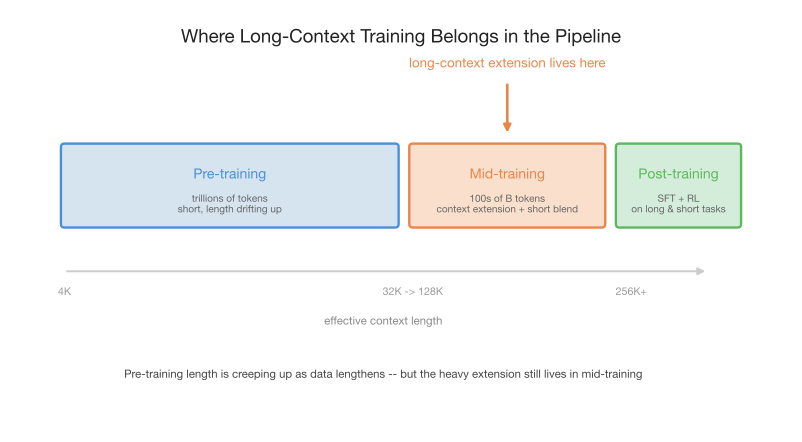
Figure 1. Bulk pre-training stays short and cheap; context extension happens in mid-training; both mid-training and post-training work to preserve short-context ability. The long-context window is grown where it's relatively cheap to grow.
Mid-training has emerged as a distinct stage between pre-training and post-training — a computational middle ground for objectives like domain expansion, context extension 1, and laying the groundwork for later reinforcement learning. OLMo 2 2 helped establish it as a load-bearing part of the modern pipeline. The recipe is almost universal now: pre-train the bulk at short context, then extend the window in mid-training on a curated mixture that keeps enough short data in the blend to hold short-context ability steady.
The dominant pattern is progressive, multi-stage extension. You don’t jump from 8K to 1M in one step — you climb a ladder, and (the pre-training drift above notwithstanding) most of that climb still happens in mid-training.
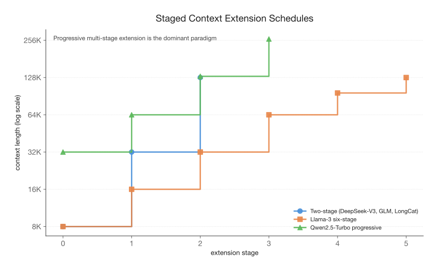
Figure 2. Three real schedules. A coarse base→32K→128K climb is the common baseline; Llama-3 uses a granular six-stage climb; Qwen-2.5-Turbo pushes progressively to 256K. All share the same shape: roughly multiply the window, stabilize, repeat — adding rungs as 1M+ targets become standard.
Multi-stage extension (base → 32K → 128K, and increasingly on to 1M+) is the norm — DeepSeek-V3, GLM-4.5, and our own LongCat-Flash all climb this way 3. As 1M-token windows become table stakes, the ladder simply grows more rungs. Llama-3 4 takes the most granular path: six increments from 8K to 128K, and notably the schedule is milestone-gated rather than fixed — it advances to the next length only once the model has both recovered its short-context scores and solved needle-in-a-haystack at the current length — spending roughly 800B tokens on extension in total. Qwen-2.5-Turbo 5 climbs progressively through 32K → 64K → 128K → 256K. Smaller open models follow the same shape: xGen-small 13 pre-trains at 4K with RoPE base 10K, then in a final stage raises the base to ~1.3×10⁸ and trains on sequences up to 256K to land a stable 128K window — quality-annealing first, length-extending second.
How many tokens does extension actually cost? Less than you’d fear. Fu et al. 6 showed 500M–5B well-curated tokens suffice for 128K. ProLong 7 reached 512K capability using only ~5% of Llama-3.1’s long-context budget. Llama-3’s 800B is the high end; Phi-4 8 used ~250B. The lesson: context extension is cheap relative to pre-training, as long as you do it as a dedicated stage rather than smearing it across the whole run. That said, the budget is creeping up: as more downstream trajectories — agent traces, long tool-use sessions — flow into mid-training to set up a strong base for later RL, the data volume at this stage is growing with them.
Opinionated default. Keep bulk pre-training short — but don’t be dogmatic; let the natural length of your data set the floor → extend in a dedicated mid-training stage along a progressive ladder (multiply the window each step, by 2-4×, not necessarily exactly double) → keep short data in the blend throughout so short-context ability never slips. Don’t try to reach your final window in one giant leap.
Ingredient 2: Data — Composition and Balance
Once you know when and where to extend, the question becomes what to feed. This is where most of the real engineering lives, and where the most expensive trial-and-error happens.
The single most important number in long-context data is the long/short ratio. The intuition that trips people up: you cannot train on all-long data. Do that, and the model catastrophically forgets short-context ability and suffers distribution shift. The shift isn’t that long data is less diverse — in some ways it’s richer, full of books, repositories, and multi-document clusters — it’s that its composition differs sharply from the pre-training mix: genres like long-form fiction, legal text, and whole codebases are over-represented relative to the short web snippets the model saw most. Train only on that and the model drifts toward those genres and regresses elsewhere. Qwen-2.5 5 settled on 40% long sequences at the current target length, 60% shorter sequences. The 60% short isn’t filler; it’s what keeps the model anchored to everything it already knew. Treat 40/60 as a starting point, not gospel — and note it needn’t be a single binary split: you can bucket by length (e.g. separate 8K / 32K / 128K pools) and tune the share of each, since the right mixture differs across models and across the rungs of one extension ladder. It’s a knob to tune, not a constant to copy.
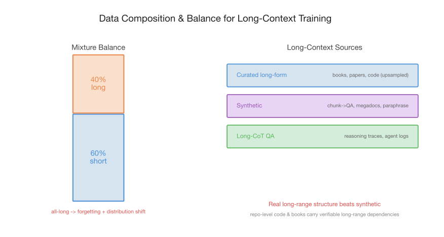
Figure 3. The 40/60 long/short balance keeps short-context ability intact while teaching long-range dependency. Long data comes from three sources, and synthetic must be used sparingly.
Where does the long data come from? Three sources, in rough order of trustworthiness:
- Curated long-form text — books, papers, legal filings, and code with genuine cross-file dependencies. Repository-level code is especially valuable: its import graphs and cross-file references encode real, verifiable long-range structure that synthetic data struggles to imitate. In practice the rarest of these are upsampled (repeated) to fill the length budget — cheap, but over-repetition risks memorization.
- Synthetic data — chunk-and-QA (pick the salient chunks of a document, generate QA pairs over them, and append the pairs 9 — a recipe production models like NVIDIA’s Nemotron Nano 2 12 adopt directly), megadocs that stitch related sources into long sequences with controlled dependencies 10, and paraphrasing that teaches retrieval through rephrasing 11.
- Long-CoT QA and trajectories — reasoning traces, multi-turn tool-use sessions, long-horizon agent logs. Increasingly important as models move toward agentic work.
A sharp caution on synthetic: relying solely on synthetic data exacerbates hallucination and degrades knowledge-intensive performance 1. Synthetic data teaches the shape of long-range retrieval, but it can’t substitute for the factual density of real text. Use it to fill the length distribution, not to replace the corpus.
This connects back to a tension I raised in the Ultra-Long Context Paradox: the impossible triangle of quality, diversity, and length. Any two are easy; all three at once, at 1M scale, is the data-engineering problem most worth caring about behind every long-context model. The long/short ratio and the three sources are both tactics for buying back what the triangle takes away.
Opinionated default. Start near 40% long / 60% short and tune per model and per stage — it’s not a universal constant. Lead with curated real long-form; use synthetic to fill the length tail, never as the backbone.
A note on post-training data, since it surprises people: you don’t necessarily need long sequences everywhere downstream. Short-context SFT largely preserves the long-context ability you built in mid-training — the model rarely forgets how to attend far just because its instruction data is short. RL is the exception. Long-context RL is genuinely harder: rollouts over 100K-token prompts are slow and memory-hungry, rewards over long horizons are noisier, and the on-policy distribution can drift away from the long inputs you care about. Many teams sidestep it by doing RL mostly at short context and relying on generalization, but if long-horizon behavior is the actual product (deep research, agentic coding), you eventually have to pay for long-context RL directly — a topic large enough to deserve its own post.
Ingredient 3: Extrapolation — Cheating the Length Tax
Here’s the dream: train short, test long. If you could train at 32K and have the model just work at 128K, you’d dodge most of the cost. You can’t get all the way there — but you can get surprisingly far, and the lever is almost embarrassingly simple.
That lever is the RoPE base frequency. Rotary position embeddings encode position by rotating query and key vectors; the embedding dimensions are split into pairs, and each pair rotates at its own frequency, geometrically spaced from fast to slow by a base parameter (classically 10,000). The fast (high-frequency) pairs spin through many full cycles within a short window and capture local offsets; the slow (low-frequency) pairs barely complete a fraction of a turn across the whole sequence and carry long-range position. The problem with extrapolation is the slow end: at positions longer than training, those low-frequency pairs reach rotation angles the model never saw, so the dot product between far-apart tokens lands in unfamiliar territory and looks like noise. The fix, Adjusted Base Frequency (ABF) 14, is just to raise the base: a larger base slows every frequency, lengthening each pair’s period so the same absolute distance maps to a smaller, already-seen rotation angle. Bigger base → slower rotation → longer effective period → more reach. This high-frequency-local / low-frequency-global split is the lens for everything below.
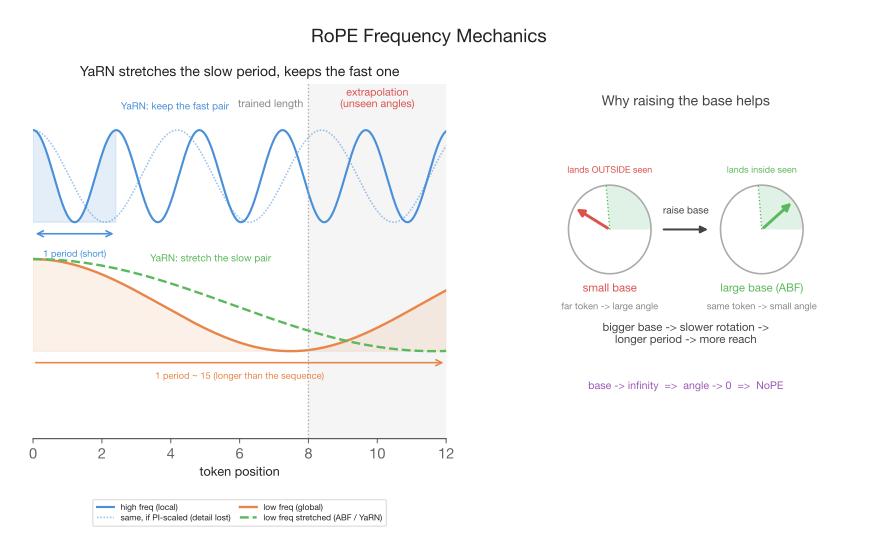
Figure 4. Left: high-frequency dimension pairs complete many cycles inside the trained window (one short period shaded in blue), while low-frequency pairs barely turn — their period (shaded orange) is longer than the whole sequence — so they carry long-range position. The selective trick: YaRN (and ABF/NTK) stretches the slow low-frequency period (green dashed) while keeping the fast high-frequency one as-is; a uniform PI scaling instead stretches even the fast pairs (dotted blue) and loses local detail. Right: the green wedge is the range of rotation angles seen during training; under a small base a far token rotates *past* it (unseen, looks like noise), while a larger base (ABF) keeps the same token inside the seen range. Push the base to infinity and the angle collapses to zero — that limit is NoPE.
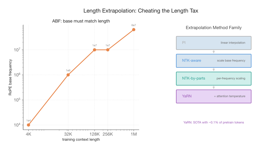
Figure 5. Left: the RoPE base must scale with training length — 10K at 4K, 1M at 32K, 10M+ past 256K. Right: the method family, from naive linear interpolation (PI) up to YaRN, which adds attention-temperature scaling and reaches SOTA with ~0.1% of pre-training tokens.
The critical, under-appreciated point is on the left of Figure 5: the base must match the training length. This isn’t a free knob you crank to infinity. Qwen-2.5 raises the base from 10,000 to 1,000,000 when extending to 32K, and to 10,000,000 past 256K 5. ProLong 7 found that keeping Llama-3’s stock 500,000 base at 512K training length degrades performance — Dynamic NTK suggested ~64,000,000 instead. Too small a base for your length, and long-range positions collapse together; the base and the length are coupled.
There’s a family of methods refining the raw base bump:
- Position Interpolation (PI) 15 — linearly squeeze positions into the trained range. Simple, but uniform scaling crushes high-frequency (local) detail.
- NTK-aware 16 — scale the base nonlinearly, by a factor of td/(d-2) for length ratio t and head dim d. Preserves high frequencies better than PI.
- NTK-by-parts — scale different frequency bands differently; leave high-frequency (local) slots alone, stretch only the low-frequency (long-range) ones. The reason: high-frequency dimensions already complete many rotations within the trained window, so the model has seen their full range and they extrapolate fine — it’s the slow, low-frequency dimensions that never finish a cycle and need interpolating.
- YaRN 17 — NTK-by-parts plus an attention-temperature correction (the softmax logits contract as context grows; temperature counters it). YaRN reaches SOTA context extension fine-tuning on ~0.1% of the original pre-training tokens, in a few hundred steps.
All four are reading off the same frequency picture from Figure 4 — and the key axis between them is uniform vs. selective. PI scales the position indices, which scales every frequency by the same factor, so it squeezes the high-frequency local pairs the model never needed squeezed (Figure 4’s dotted blue wave — local detail distorted for no benefit). ABF does the opposite: it raises the base, and because each pair’s frequency is base^(−2i/d), a larger base barely moves the fastest pairs while slowing the slow ones the most. So ABF is not a uniform version of PI — it’s already frequency-selective, mechanically the same move as NTK-aware. NTK-by-parts makes the selectivity explicit with a hard band split (leave the fast pairs alone, interpolate only the slow ones), and YaRN adds the attention-temperature fix on top. The progression is PI (uniform, crude) → ABF ≈ NTK-aware (selective via the base) → NTK-by-parts (explicit band split) → YaRN (+ temperature) — each a smarter way to stretch the slow period without touching the fast one.
A natural question: why patch RoPE at all — why not drop positional encodings entirely? NoPE (no positional encoding) 25 leans on the causal mask alone to encode order, and it does generalize past its training length somewhat better than vanilla RoPE. But it isn’t a free win. NoPE eventually fails the same way, through attention dispersion (heads spread their weight evenly once they run past familiar lengths), and on perplexity it still trails a well-tuned YaRN. RoPE also retains something NoPE provably cannot build — arbitrarily sharp, purely positional attention — which matters for local structure. So the field has mostly landed on hybrids: keep RoPE in local/sliding-window layers, drop it in a fraction of global layers (e.g. every fourth), getting NoPE’s long-range reach without losing RoPE’s local precision. NoPE is a design knob within the stack, not a replacement for the extrapolation toolkit above.
It’s worth contrasting two flavors of “hybrid,” because they’re easy to conflate. The NoPE-RoPE hybrid splits which layers get positional information at all — RoPE in the local layers, none in selected global ones. MiMo-V2-Flash 21 does something subtler within a hybrid attention design (39 sliding-window layers to 9 global, a 5:1 ratio, 128-token window): it keeps RoPE everywhere but tunes it per role. RoPE is applied partially — only to the first 64 query/key dimensions, leaving the rest position-free — and the RoPE base differs between the SWA and global layers: a small base suits the 128-token local window, while the global layers need a much larger base to span the full sequence. The takeaway is the same lens as before: the high-frequency/local and low-frequency/global split isn’t just a property of one RoPE setting, it’s a knob you can set differently for different layers depending on the range each layer is responsible for.
And the two flavors aren’t really separate — they’re endpoints of one axis. Look again at the right of Figure 4: raising the base shrinks every rotation angle. Push the base to infinity and every angle goes to zero — the rotations vanish and RoPE becomes a no-op. NoPE is just RoPE with an infinite base. So “drop positional encoding in the global layers” and “give the global layers a much larger base” are the same move in different costume: both flatten the long-range rotation so far-apart tokens stop looking like noise. That’s why partial RoPE, per-layer base tuning, and NoPE-in-some-layers all coexist in modern hybrids — they’re sliding the same dial.
The counterintuitive result that ties it together: a short fine-tune with an adjusted base can extrapolate far beyond its training length. Code Llama 18 set the base to 1,000,000, trained at 16K, and reached 100K+. The base-scaling literature 16 shows fine-tuning at 4K-16K with the right base can extrapolate to 100K.
But — and this is the part I want to push on — extrapolation buys reach, not reliability. A model that extrapolates to 128K will answer questions there, but its precision in the middle of that window (the context rot I described in the Paradox post) is worse than a model that genuinely trained at 128K. Extrapolation is a discount, not a free lunch. Use it to stretch past your training length cheaply, but if 128K is your product spec, do at least some real training at 128K.
Opinionated default. Use ABF, with the base matched to each stage’s length (not a fixed value). Reach for YaRN when you need cheap extension on a small token budget. You can ship a window you only ever extrapolated to — it just tends to be measurably weaker than one you trained at the target — so if a length matters for your product, spend at least some real training there.
Ingredient 4: Parallelism — The Systems Tax
The first three ingredients are about modeling. This one is about whether you can afford to run the recipe at all. A 1M-token sequence does not fit on one device — the activations alone overflow HBM — so you must shard the sequence itself across GPUs. That’s context parallelism (CP).
I covered the evolution of CP in the Ultra-Long Context Paradox — Ring Attention → DeepSpeed Ulysses → Llama-3’s all-gather → today’s hybrid intra/inter-node schemes. I won’t re-run that history here. Instead, the recipe-level things you actually need to get right:
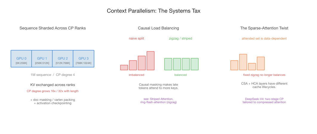
Figure 6. Left: the sequence is sharded across CP ranks, which exchange KV; CP degree climbs with length. Middle: causal masking makes a naive split badly imbalanced — late tokens attend to far more keys — and zigzag/striped assignment evens the per-rank work. Right: under sparse attention the attended set is data-dependent, so a fixed split no longer balances — DeepSeek-V4 uses a two-stage CP tailored to its compressed layers.
Know when you need it. CP degree grows with context — 16×, 32×, and beyond — and it competes with your other parallelism dimensions for the device budget. You don’t pay this tax at 8K; you pay it sharply once you’re extending to 128K+. Budget for it when you plan the extension stages, not after.
Pack and mask correctly. Long-context batches are full of variable-length documents. Naive padding wastes enormous compute at these lengths, so you pack documents and use variable-length (varlen) attention with proper document masking — so tokens don’t attend across document boundaries. Combined with activation checkpointing, this is what keeps memory tractable. It’s also a structural reason long-context training doesn’t belong in bulk pre-training: when the corpus is overwhelmingly short, a long window spends most of its compute on packed-together fragments with masked-off cross-document attention — you pay the quadratic cost of a long sequence while only ever attending within short spans. The long window earns its keep only once the data is genuinely long, which is exactly why extension waits for a dedicated stage.
Balance the causal load. This is the subtle one. Causal masking means token i attends to all tokens ≤ i — so if you split the sequence into contiguous chunks across ranks, the rank holding the last chunk does far more attention work than the rank holding the first. A naive split is badly imbalanced (Figure 6, middle). The fix is to assign tokens to ranks in a zigzag / striped pattern so every rank gets a mix of early and late positions, evening the work — the trick introduced by Striped Attention 23, with the de facto reference implementation being the zigzag varlen kernel in ring-flash-attention 26. (A naming caveat to avoid confusion: our own LongCat ZigZag Attention 19 borrows the word “zigzag” for a different idea — a structured sparse attention pattern retrofitted during continued pre-training — not this CP load-balancing scheme. Full disclosure: that’s my work.) The broader point stands regardless of method: at long context, load balancing across CP ranks is not an optimization, it’s the difference between training in days and training in weeks. Efficient ultra-long training frameworks — e.g. the 128K-to-4M recipe of Xu et al. 20 — are largely engineering victories of exactly this kind.
It helps to see why the CP schemes differ, in terms of what each one moves and computes. For a sequence of length n sharded over a CP degree of p:
| Scheme | Per-step communication | What’s communicated | Trade-off |
|---|---|---|---|
| Ring (P2P) | O(n/p) per hop, p hops | KV blocks passed around the ring | Overlaps comms with compute, but latency grows with p |
| Ulysses (all-to-all) | O(n/p) per all-to-all | tokens ↔ heads re-layout | Cheap bandwidth, but CP degree capped by #KV heads |
| All-gather (Llama-3) | O(n) gathered KV | full KV tensors to every rank | Simple, trades memory for one big collective |
The causal-masking imbalance sits on top of all three: whichever scheme you pick, a contiguous split leaves late ranks doing up to ~2× the FLOPs of early ranks, which is the slack zigzag assignment recovers.
Mind the sparse-attention twist. Everything above assumes dense attention. Once the model is sparse, CP changes shape. With a smaller KV footprint the communication-heavy hybrid schemes matter less, but the load-balancing problem gets harder, not easier: which tokens each query attends to is now data-dependent, so a fixed zigzag split no longer guarantees even work. DeepSeek-V4 22 is the worked example — its compressed-sparse (CSA) and heavily-compressed (HCA) layers each have different cache lifecycles, so it adopts a two-stage contextual parallelism tailored to compressed attention rather than a single uniform CP scheme. The lesson: your parallelism plan is coupled to your attention architecture, and a sparse model needs a CP strategy designed for it, not inherited from the dense recipe.
Opinionated default. Hybrid CP (all-to-all within node, point-to-point across nodes) for dense attention — though with sparse attention’s smaller KV footprint, a simpler all-gather scheme becomes acceptable again. Add varlen packing with document masking, activation checkpointing, and zigzag load balancing for the causal mask. Plan the CP degree into your extension stages from the start.
The North Star: Evaluation
The four ingredients tell you how to build a long-context model. Evaluation tells you whether you succeeded — and it’s where the most self-deception happens, so it deserves to sit alongside the recipe rather than as an afterthought.
The trap is the single-needle needle-in-a-haystack (NIAH) test. It’s easy to run and easy to ace — modern models score ~100% — which is exactly why it’s nearly useless as a discriminator. Passing single-needle NIAH tells you the model can copy one fact across distance; it says almost nothing about whether the model can reason over a long context. The number that actually matters is effective context length: the length at which the model still performs, not the length printed on the box. RULER 28 made this gap concrete — extending NIAH with multi-hop tracing, aggregation, and multi-needle retrieval, it showed that most models advertising 32K+ collapse well before their claimed window. The lesson generalizes: claimed and effective length routinely differ by an order of magnitude.
So, a few rules I’d hold any long-context model to:
- Test at your real working length, with multi-needle tasks. Single-needle scores overstate production capability badly. If your application cross-references several facts across 128K, evaluate exactly that.
- Watch the middle, not just the ends. The lost-in-the-middle effect (from the Paradox post) means accuracy dips for information placed mid-context; report positional variance, not just an average.
- Map benchmarks to the atomic abilities they test. “Long-context ability” isn’t one skill — it decomposes into a few atomic capabilities, and each benchmark targets a different one. No single test covers them all; triangulate.
| Atomic ability | What it means | Probed by |
|---|---|---|
| Retrieval | locate a fact (or several) across distance | NIAH (single), RULER multi-key 28 |
| Multi-hop reasoning | chain references that can’t be solved sequentially | GraphWalks 31, RULER multi-hop tracing |
| Aggregation | collect & summarize information spread across the window | RULER aggregation 28 |
| Abstraction | synthesize long input into new, condensed text (not copy spans) | HELMET summarization 33, LongBench v2 29 |
| Disambiguation | tell apart repeated, near-identical items | MRCR 30 |
| Realistic comprehension | RAG, multi-doc QA, summarization on natural text | HELMET 33, LongBench v2 29 |
| Code understanding | reason over a repository-scale codebase | LongCodeBench 32 — LongCodeQA (comprehension) + LongSWE-Bench (repair) |
RULER’s synthetic design is the workhorse — it isolates context ability from memorized knowledge and lets you dial length precisely — but synthetic retrieval overstates real capability, so pair it with realistic suites (HELMET, LongBench v2) and the reasoning-heavy probes (GraphWalks, MRCR) before trusting a number.
The reason to think in atomic abilities is that downstream evals compose them. A “deep research” task is retrieval + multi-hop + aggregation over realistic documents; agentic coding is code understanding + multi-hop across files + disambiguation of similar symbols; long-dialogue assistants lean on disambiguation + retrieval over a growing history. When an application-level eval regresses, decomposing it back into atomic abilities tells you which ingredient of the recipe to revisit — a retrieval failure points at the long/short ratio or RoPE base; an aggregation failure at mid-context positional handling; a code failure at the repository data in your mixture. The atomic benchmarks are the diagnostic layer beneath the application benchmarks.
Worth watching, too, are reasoning benchmarks that aren’t nominally about length at all. In the Ultra-Long Context Paradox I noted context grokking — that reasoning scores on tasks like AIME can jump once context scaling crosses a threshold, as if the capacity to hold more state and the capacity to reason over it unlock together. So a short-prompt reasoning benchmark like AIME doubles as an indirect health check on long-context training: a model whose long-context recipe is working often shows gains there too, even though the prompts are short.
- Guard short context. Every extension stage should re-check short-context scores — Llama-3’s milestone gating did exactly this. A model that gains 128K but loses 4K isn’t an upgrade.
Evaluation is the feedback loop that closes the recipe: it’s how you set the long/short ratio, decide whether extrapolation is good enough, and know when a stage has actually converged. Build it first, not last.
The Reference Recipe
Putting the four ingredients together, here’s the end-to-end default I’d reach for — the thing I’d actually do, absent a specific reason to deviate.
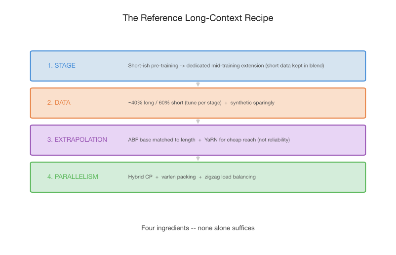
Figure 7. The four ingredients as one recipe. Each addresses a different failure mode; skip any one and the model is slow, forgetful, short-sighted, or untrainable.
| Ingredient | Default | Failure it prevents |
|---|---|---|
| Stage | Short-ish pre-training (let data set the floor) → dedicated mid-training extension on a progressive ladder, short data kept in the blend | Wasted quadratic compute; short-context regression |
| Data | ~40% long / 60% short, tuned per model and stage; real long-form first, synthetic to fill the tail | Forgetting, distribution shift, weak long-range signal |
| Extrapolation | ABF with base matched to length; YaRN for cheap reach; real training at the target for reliability | Position collapse; reach without precision |
| Parallelism | Hybrid CP, varlen packing + doc masking, activation checkpointing, zigzag load balancing — and a CP scheme matched to your attention (sparse models need their own) | Out-of-memory; weeks-long training from CP imbalance |
The reason none of these is optional: each guards a different failure mode. Skip staging and you burn compute. Skip data balance and you forget. Skip extrapolation discipline and your window is hollow. Skip parallelism engineering and you simply can’t run the job. They interact, too — your extrapolation base depends on your staged lengths; your CP budget depends on those same lengths; your data ratio shifts as the window grows.
What’s Actually Hard
If there’s a single thread through all four ingredients, it’s that data and systems engineering now carry as much weight as the architecture. That’s not to diminish architecture — all four ingredients matter, and a bad attention design will sink you regardless. But the attention mechanism is increasingly a shared, reproducible asset: the sparse architectures from the Landscape post are mature and converging, and they transfer across labs cheaply. GLM-5 27 reproduced DeepSeek’s sparse attention via continued pre-training on only ~20B tokens — a few percent of a from-scratch budget. What’s harder to copy is the rest of the recipe: the long/short ratio, the base-frequency schedule, the document masking, the load balancing. The folklore.
I find that genuinely encouraging. A model architecture, once published, can be reproduced in weeks — GLM cloning DSA is proof. Data and systems engineering is harder to hand off but eminently learnable — it rewards care, measurement, and the kind of accumulated craft that this post is trying, in a small way, to write down. The recipe isn’t secret. It’s just scattered. And now, at least the outline of it is in one place.
References
[1] Chengying Tu et al. A Survey on LLM Mid-Training. arXiv:2510.23081, 2025.
[2] Team OLMo. 2 OLMo 2 Furious. arXiv:2501.00656, 2025.
[3] DeepSeek-AI. DeepSeek-V3 Technical Report. arXiv:2412.19437, 2024.
[4] Aaron Grattafiori et al. The Llama 3 Herd of Models. arXiv:2407.21783, 2024.
[5] Qwen Team. Qwen2.5 Technical Report. arXiv:2412.15115, 2024.
[6] Yao Fu et al. Data Engineering for Scaling Language Models to 128K Context. arXiv:2402.10171, 2024.
[7] Tianyu Gao et al. How to Train Long-Context Language Models (Effectively). arXiv:2410.02660, ACL 2025.
[8] Marah Abdin et al. Phi-4 Technical Report. arXiv:2412.08905, 2024.
[9] Linda He, Jue Wang, Maurice Weber, Shang Zhu, Ben Athiwaratkun, and Ce Zhang. Scaling Instruction-Tuned LLMs to Million-Token Contexts via Hierarchical Synthetic Data Generation. arXiv:2504.12637, ICLR 2025.
[10] Konwoo Kim et al. Data-Efficient Pre-Training by Scaling Synthetic Megadocs. arXiv:2603.18534, 2026.
[11] Yijiong Yu et al. Training With Paraphrasing the Original Text Teaches LLM to Better Retrieve in Long-Context Tasks. arXiv:2312.11193, 2023.
[12] NVIDIA. Nemotron Nano 2: An Accurate and Efficient Hybrid Mamba-Transformer Reasoning Model. arXiv:2508.14444, 2025.
[13] Erik Nijkamp, Bo Pang, Egor Pakhomov, Akash Gokul, Jin Qu, Silvio Savarese, Yingbo Zhou, and Caiming Xiong. xGen-small Technical Report. arXiv:2505.06496, 2025.
[14] Wenhan Xiong et al. Effective Long-Context Scaling of Foundation Models. arXiv:2309.16039, NAACL 2024.
[15] Shouyuan Chen et al. Extending Context Window of Large Language Models via Positional Interpolation. arXiv:2306.15595, 2023.
[16] Xiaoran Liu et al. Scaling Laws of RoPE-based Extrapolation. arXiv:2310.05209, ICLR 2024.
[17] Bowen Peng et al. YaRN: Efficient Context Window Extension of Large Language Models. arXiv:2309.00071, 2023.
[18] Baptiste Rozière et al. Code Llama: Open Foundation Models for Code. arXiv:2308.12950, 2023.
[19] Chen Zhang et al. Efficient Context Scaling with LongCat ZigZag Attention. arXiv:2512.23966, 2025.
[20] Chejian Xu et al. From 128K to 4M: Efficient Training of Ultra-Long Context Large Language Models. arXiv:2504.06214, 2025.
[21] LLM-Core Xiaomi. MiMo-V2-Flash Technical Report. arXiv:2601.02780, 2026.
[22] DeepSeek-AI. DeepSeek-V4 Technical Report. HuggingFace, 2026.
[23] William Brandon, Aniruddha Nrusimha, Kevin Qian, Zachary Ankner, Tian Jin, Zhiye Song, and Jonathan Ragan-Kelley. Striped Attention: Faster Ring Attention for Causal Transformers. arXiv:2311.09431, 2023.
[24] Microsoft AI. MAI-Thinking-1: Building a Hill-Climbing Machine. microsoft.ai, 2026.
[25] Amirhossein Kazemnejad, Inkit Padhi, Karthikeyan Natesan Ramamurthy, Payel Das, and Siva Reddy. The Impact of Positional Encoding on Length Generalization in Transformers. arXiv:2305.19466, NeurIPS 2023.
[26] Zilin Zhu et al. ring-flash-attention: Ring Attention with FlashAttention (zigzag varlen implementation). GitHub, 2024.
[27] Zhipu AI. GLM-5: from Vibe Coding to Agentic Engineering. arXiv:2602.15763, 2026.
[28] Cheng-Ping Hsieh et al. RULER: What’s the Real Context Size of Your Long-Context Language Models? arXiv:2404.06654, COLM 2024.
[29] Yushi Bai et al. LongBench v2: Towards Deeper Understanding and Reasoning on Realistic Long-context Multitasks. arXiv:2412.15204, 2024.
[30] OpenAI. MRCR: Multi-Round Co-reference Resolution. HuggingFace, 2025. Building on the Gemini MRCR eval (arXiv:2409.12640).
[31] OpenAI. GraphWalks: Multi-Hop Long-Context Reasoning (released with GPT-4.1). HuggingFace, 2025.
[32] Stefano Rando, Luca Romani, Alessio Sampieri, Luca Franco, John Yang, Yuta Kyuragi, Fabio Galasso, and Tatsunori Hashimoto. LongCodeBench: Evaluating Coding LLMs at 1M Context Windows. arXiv:2505.07897, 2025.
[33] Howard Yen, Tianyu Gao, Minmin Hou, Ke Ding, Daniel Fleischer, Peter Izsak, Moshe Wasserblat, and Danqi Chen. HELMET: How to Evaluate Long-Context Language Models Effectively and Thoroughly. arXiv:2410.02694, ICLR 2025.